Metode Runge-Kutta
Metode Runge-Kutta
Metode Deret Taylor (MDT) memiliki error lokal yang bergantung dengan tingginya order \(O\left(h^{m+1} \right)\), dimana \(m\) adalah order MDT. Ini berarti jika kita ingin hasilnya mendekati solusi eksak maka kita harus menggunakan MDT order tinggi. Namun kendala yang dihadapi adalah kita harus mencari turunan order tinggi \(y'',y''',\dots\) yang mana sulit untuk didapatkan dan memakan waktu komputasi yang tidak sedikit.
Contoh 2. Terapkan Metode RK 2 dan 4 untuk
\[
\begin{matrix}
y' = -y + e^{-t}, & y(0)=0.
\end{matrix}
\]
(Solusi eksaknya adalah \(y(t)=te^{-t}\).)
import numpy as np
import math
import matplotlib.pyplot as plt
%matplotlib inline
def f(t, y):
    #k = 6.22e-19
    #n1 = 2e3
    #n2 = 2e3
    #n3 = 3e3
    #return (k*((n1 - y/2)**2)*((n2 - y/2)**2)*((n3 - 3*y/4)**3))
    #return -y + math.exp(-t)
    return y - t**2 + 1
h = 0.2
T = 2
# Metode Heun / RK-2

N = int(T/h)
t = np.zeros(N+2)
y_h = np.zeros(N+2) + 0.5
y_a = np.zeros(N+2) + 0.5

for k in range(N+1):
    t[k+1] = t[0] + (k+1)*h
    #y_a[k+1] = t[k+1]*math.exp(-t[k+1])
    y_a[k+1] = (t[k+1] + 1)**2 - 0.5*math.exp(t[k+1])

    K1 = h*f(t[k], y_h[k])
    K2 = h*f(t[k+1], y_h[k]+K1)

    y_h[k+1] = y_h[k] + 0.5*(K1+K2)
# Metode RK4
N = int(T/h)
t = np.zeros(N+2)
y_rk4 = np.zeros(N+2) + 0.5


for k in range(N+1):
    t[k+1] = t[0] + (k+1)*h

    K1 = h*f(t[k], y_rk4[k])
    K2 = h*f(t[k]+0.5*h, y_rk4[k]+0.5*K1)
    K3 = h*f(t[k]+0.5*h, y_rk4[k]+0.5*K2)
    K4 = h*f(t[k]+h, y_rk4[k]+K3)

    y_rk4[k+1] = y_rk4[k] + 1/6*(K1+2*K2+2*K3+K4)
for i in range(N+1):
    print(t[i], y_a[i], y_h[i], y_rk4[i], abs(y_a[i]-y_h[i]), abs(y_a[i]-y_rk4[i]))
0.0 0.5 0.5 0.5 0.0 0.0
0.2 0.829298620919915 0.8260000000000001 0.8292933333333333 0.003298620919914952 5.287586581692594e-06
0.4 1.2140876511793646 1.2069200000000002 1.2140762106666667 0.007167651179364354 1.1440512697857841e-05
0.6000000000000001 1.648940599804746 1.6372424000000003 1.6489220170416 0.011698199804745624 1.8582763146035575e-05
0.8 2.1272295357537665 2.1102357280000006 2.1272026849479433 0.01699380775376591 2.6850805823208646e-05
1.0 2.6408590857704777 2.617687588160001 2.6408226927287513 0.023171497610476877 3.639304172642355e-05
1.2000000000000002 3.1799415386317267 3.149578857555201 3.17989417023223 0.03036268107652562 4.736839949659455e-05
1.4000000000000001 3.732400016577664 3.693686206217345 3.732340072854979 0.038713810360318845 5.994372268469661e-05
1.6 4.283483787802443 4.235097171585161 4.283409498318405 0.04838661621728235 7.428948403820357e-05
1.8 4.815176267793525 4.755618549333896 4.815085694579433 0.05955771845962943 9.057321409233765e-05
2.0 5.305471950534675 5.233054630187353 5.305363000692653 0.07241732034732173 0.00010894984202192148
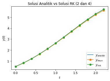
plt.title('Solusi Analitik vs Solusi RK (2 dan 4)')
plt.xlabel('$t$')
plt.ylabel('$y(t)$')

plt.plot(t,y_a, label="$y_{analitik}$")
plt.plot(t,y_h, '-o', label="$y_{heun}$")
plt.plot(t,y_rk4, '-o', label="$y_{rk4}$")
plt.legend(loc=4)
<matplotlib.legend.Legend at 0x127075f70>
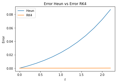
error_h = abs(y_a-y_h)
error_rk4 = abs(y_a-y_rk4)

plt.title('Error Heun vs Error RK4')
plt.xlabel('$t$')
plt.ylabel('Error')

plt.plot(t,error_h, label="Heun")
plt.plot(t,error_rk4, label="RK4")

plt.legend()
<matplotlib.legend.Legend at 0x1272d95e0>